MUSEUM OF SELF-ORGANIZATION STRUCTURES: the self-forming structures revealed by means of the computational experiment or obtained on the basis of analytical models
Russian
1. Examples of the formation of self-organizing spatial structures in flowing parts of machine-building structures and in physical devices
|
|
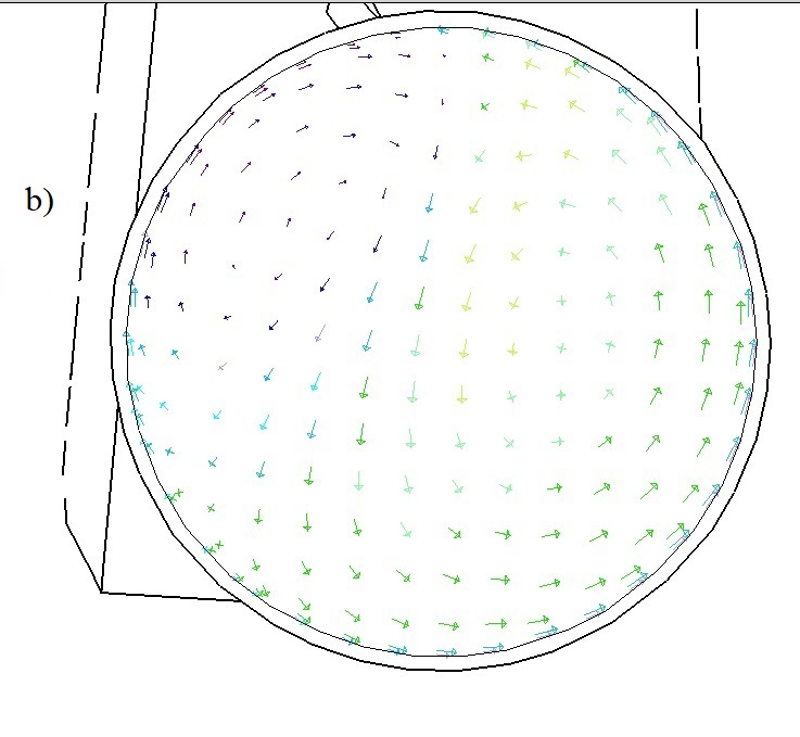
Fig. 1. The formation of the ordered spatial structure in the form of a vortex (the "stagnant region" in which air flow vortex movement occurs) at the output of the diffusor of the turbocharger TCR 6.1 compressor chamber: a) the lengthwise section b) the transverse section
|
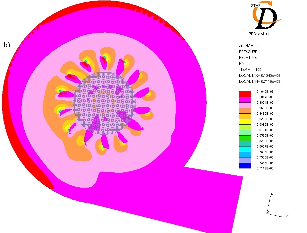
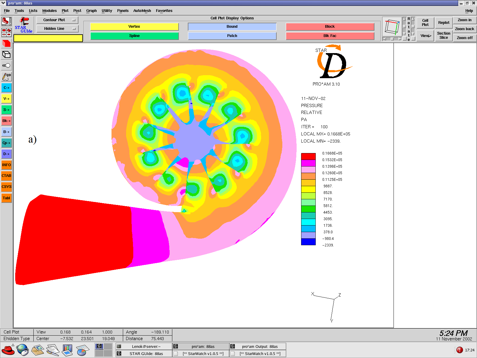
Fig. 2. The formation of ordered similar spatial structures of compression in moving continuous substance near the turbine blades into the turbocharger TCR 6.1 working chamber: a) the input velocity is 20 m/s, the outlet pressure is 10 Pa; b) the inlet pressure is 100 kPa, the outlet pressure is 98 kPa
|
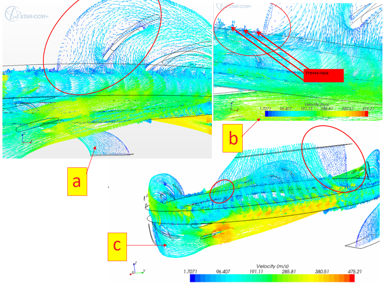
Fig. 3. The formation of self-organizing structures of the kind of the vortex zones in the moving steam-water streams described by velocity vector field of the into the acting construction of microturbine R-0.25 –1.4-250/0.6: a) at a level corresponding to the diameter D = 0.69 m (4-th level of microturbine); b) at a level corresponding to the diameter D = 0.69 m (exit system); c) at a level corresponding to the diameter of D = 0.75 m (zone of steam leakage)
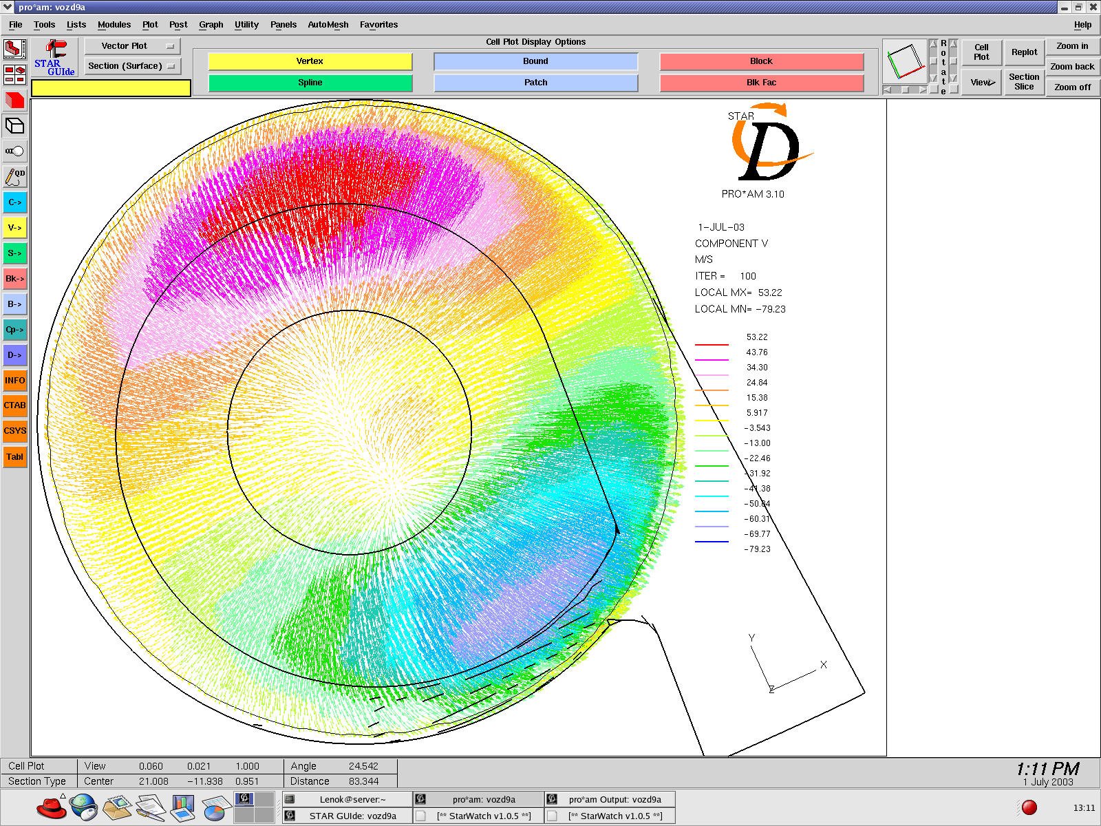
Fig. 4. The aerodynamic flow singularity formation in the form of a flat dipole in the compressor chamber of a turbocharger TCR-9 after numerical simulation (y–projection of the outlet velocity is 45 m/s, the inlet pressure is 96 kPa)
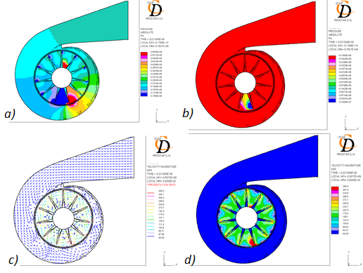
Fig. 5. The aerodynamic shock wave formation in the flowing part of the TCR-6.1 turbocharger in result of the turbine rotation process computer simulation (rotation speed is 90,000 rpm, inlet and outlet pressures, 160 kPa and 100 kPa respectively): a), b) the pictures of pressure distribution; с), d) the pictures of speed distribution
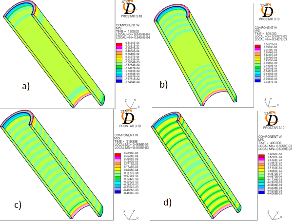
Fig. 6. The computational experiment stages of the formation in the moving fluid of Taylor vortices (Eckman cells and laminar spiral vortices) in a system of coaxial cylinders, the inner of which rotates with frequency: a) n = 1 rpm; b) n = 2 rpm; c) n = 2.3 rpm; d) n = 2.6 rpm
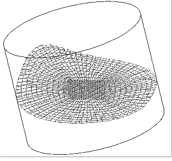
Fig. 7a. Computer simulation of the vibrational fluid movement and origin of self-organization processes leading to rotational movement of water in a vibrating tank
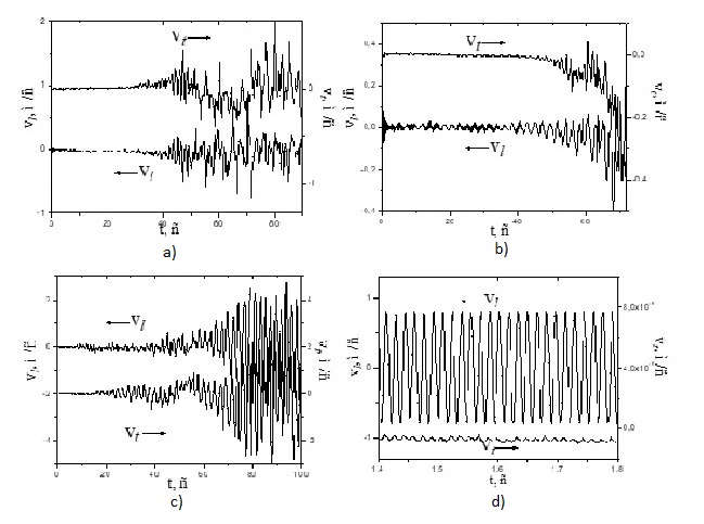
Fig. 7b. The time dependences of the transverse and longitudinal velocity components at different levels of the reservoir filling: a) one quarter, b) half, c) three quarters, d) full tank (vt is a velocity component perpendicular to the constraining force, vl is a velocity component parallel to the direction of the constraining force, t is the time)
а)
|
б)
|
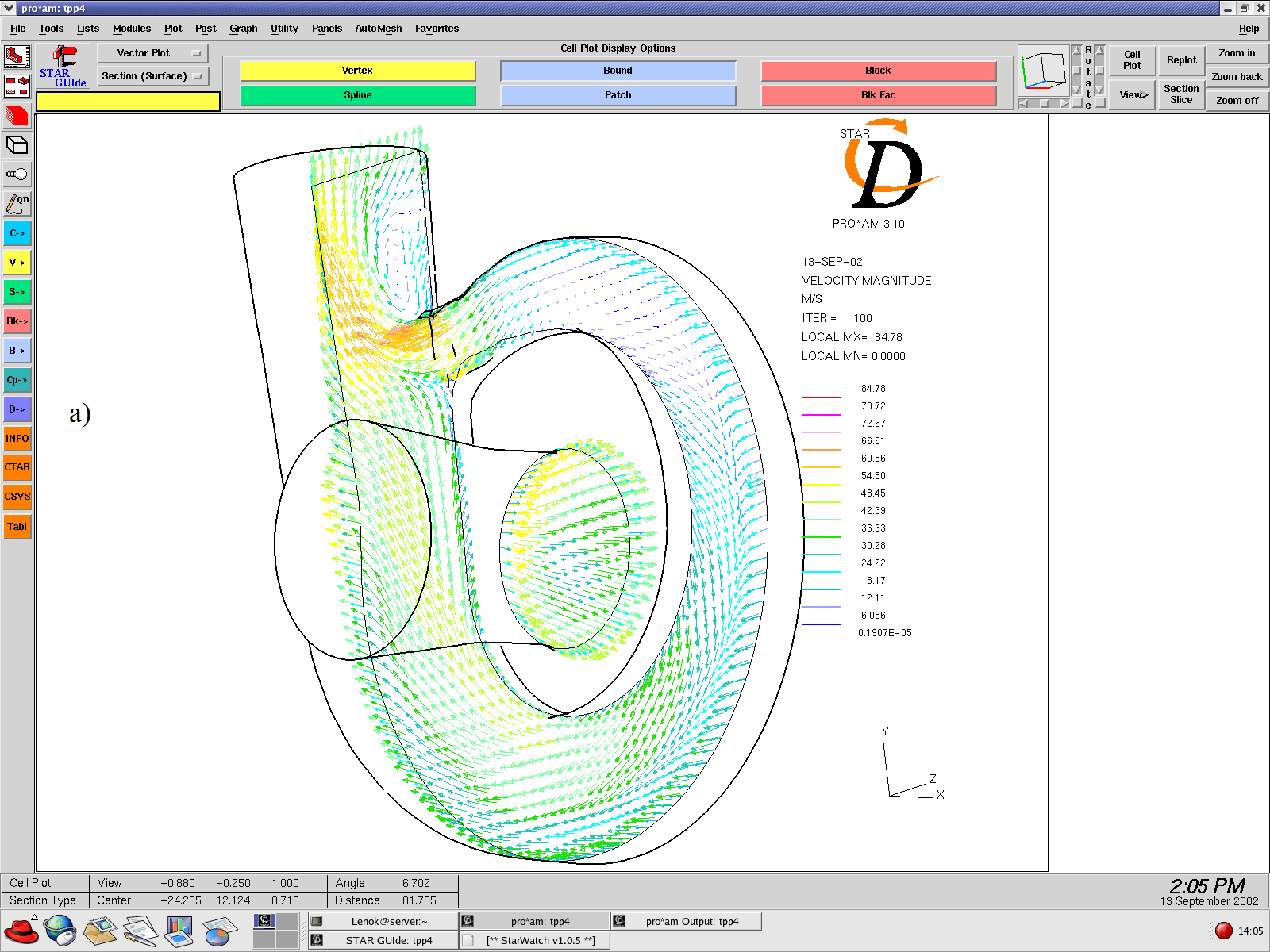
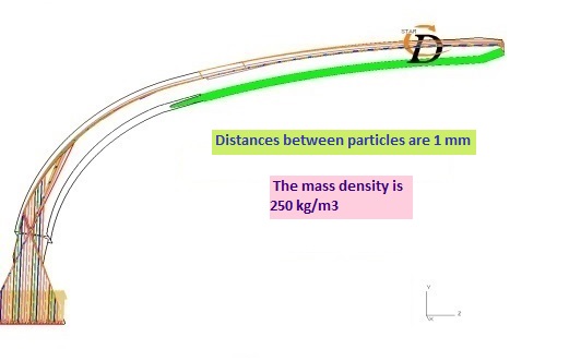
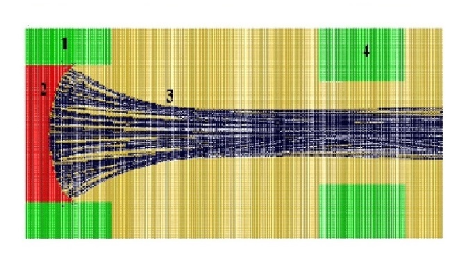
Fig. 8. The effect of self-focusing: a) of particles beam in the air flow in result of the dissipation of their kinetic energy on the walls of the curvilinear pipe of harvester based on the results of numerical experiment in STAR-CD package (particle velocity at the entrance boundary is vin (particles)
= 68.3 m/s , air flow velocity vin (air flow) = 40 m/s, particle mass density ρ = 250 kg/m3); b) of positive ions beam in an ion-optical system with a plasma emitter on the basis of modeling in the developed ELIS software complex (1 – focusing electrode with an aperture radius of 2 mm, 2 – plasma, 3 – ion beam, 4 – ion collector with an aperture radius of 1.5 mm, accelerating gap is 5 mm, accelerating voltage is 50 kV, plasma concentration is 5 × 10¹⁷ m-3)
Fig. 9. Results of the computer modeling of interaction of two kink-type solitons obtained by solution analytical of sin-Gordon equation
2. Examples of the formation of time and space-time structures in the state-space of complex systems
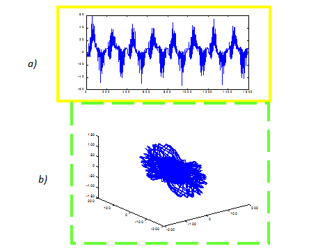
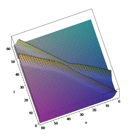
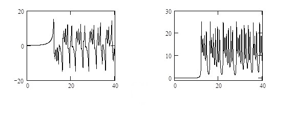
Fig. 10. The time series (a) for radial velocity component of the aerodynamic flow in the turbocompressor and its attractor representation in the state-space (b)
а)
b)
c)
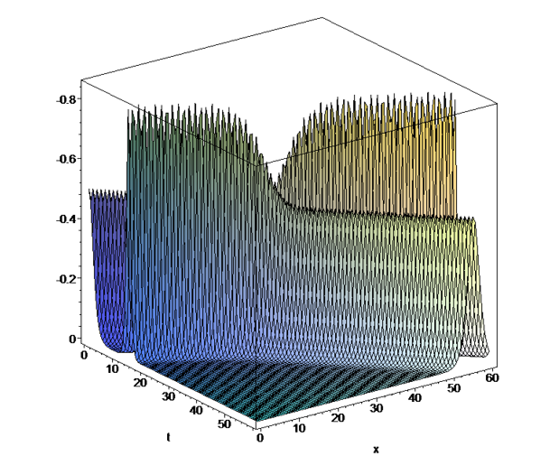
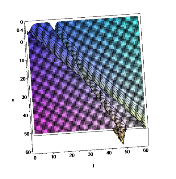
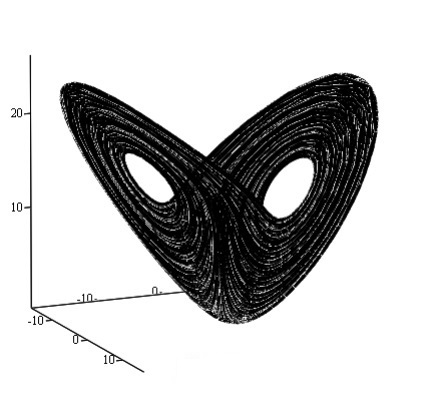
Fig. 11. A synthesized attractor describing the chaotic flow of a viscous fluid in the Couette-Taylor system in the state-space:
a) a strange attractor in the state-space with the control parameter value a = 15.0;
b) time structures describing the dependencies of the dynamic variables of system in the state-space with the control parameter value a = 15.0;
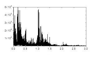
c) broadband Fourier power spectrum of dynamic variable time dependence of the system at a = 15.0 showing that the spectrum becomes continuous in a chaotic regime.
|
|
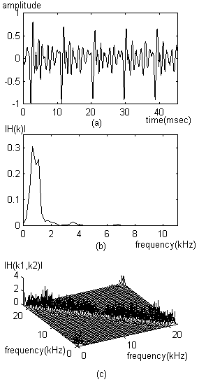
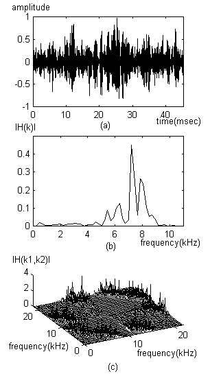
a) – the signal of the Belarusian language phoneme 'A';
b) – Wiener kernel of the first order H1 [k1] for the phoneme 'A';
c) – Wiener kernel of the second order H2 [k1, k2] for the phoneme 'A'.
|
a) – the signal of the Belarusian language phoneme 'C';
b) – Wiener kernel of the first order H1
[k1] for the phoneme 'C';
c) – Wiener kernel of the second order H2
[k1, k2] for the phoneme 'C'.
|
Fig. 12. Graphic representation of phoneme signals 'A' and 'C' in the Belarusian language
|
|
|
a)
|
b)
|
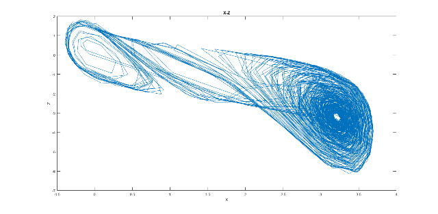
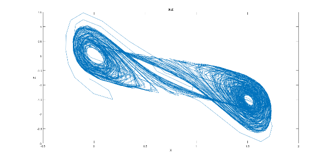
Fig. 13a. Examples of chaotic Chua’s attractor (axes X-Z) for the control parameters sets (a) and (b) obtained during five hundred iterations

Fig. 13b. Bifurcation diagram for process from the Chua's scheme for the different values of control parameters (as seen a chaotic state occurs when α=13.8,...,16.2)
|
|
|
a)
|
b)
|
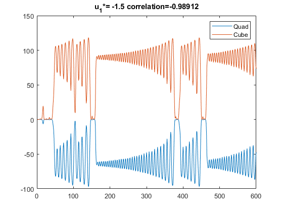
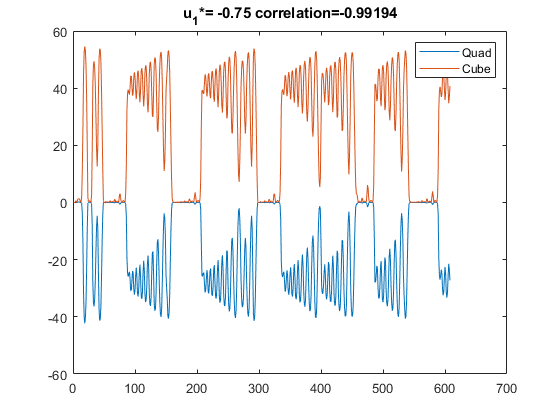
Fig. 13c. The plots of cube and quadratic terms output values of matrix series of vector function in the state-space of Chua's scheme for two sets of parameters

|
|
|
a)
|
b)
|
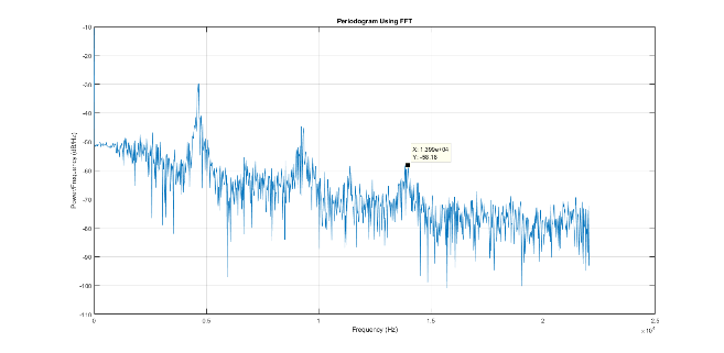
Fig. 13d. The power spectra of quasiperiodic and chaotic processes in the Chua's scheme